Sheaf Neural Networks

I describe Sheaf Neural Networks in this blog, which are a type of Graph Neural Networks.

Sheaf Neural Networks

(In progress) - I am learning about Sheaf Neural Networks and making a blog about it.

Introduction

Typical Neural Networks take in vectors as their input examples. However, there are variants such as Convolutional Neural Networks (CNNs) that take in images as their input and then process them. This heavily widens the use cases of typical Neural Netwrorks to tasks such as facial recognition, document analysis and computer vision.

Graph Neural Networks (GNNs) are also a variant of the typical Neural Networks that take in Graphs as their input. It is worth noting that such neural networks also have a great deal of potential for applications. After all, any set of objects, and connections between them are naturally expressed as a graph. We are starting to see their applications in areas such as antibacterial discovery, physics simulations, fake news detection, traffic prediction, and recommendaton systems. Images, texts, social networks, and even molecules can be represented as graphs.

However, this piece is not about going into the details of these, and I will perhaps cover them in some other piece. The one key idea I want to extract of GNNs is that we want to impose a meaningful geometric structure on graphs. Once we do so, we can apply traditional geometric principles on them making them more powerful mathematical structures (we are essentially trying to create a new category of mathematical objects which are more powerful than standard graphs). We essentially are natuarally motivated to do so, as you will see as you read on.

You impose a compatible geomtric structure on a graph through sheaves!

Understganding the question properly and the Setup

But what sort of “geometrical structure” do you want to impose? A set itself can be thought of a geometrical structure. You can take a botoom up approach to this:

Sets $->$ Topological Spaces $->$ Topological Manifolds $->$ Smooth Manifolds $->$ Riemannian Manifolds.

Each condition is stronger than the previous condition. So let us start from viewing them as topological spaces, and we will recover some of the elements of this hierarchy.

Because a graph does not have any “continuous surfaces”, we define its topology combinatorially.

Definition: The open star of a geometric element (“a cell”) is the collection of all the cells that contain it.

Here is how this global definition works for a simple graph, which just has edges and vertices.

1) The star of an edge $e$: It is just $U_e = {e}$ because there is not other cell containing it (there are no faces or other high dimensional objects in this case).

2) The star of a node $v$: A node is contained within all the edges that connect to it, as well as itself. $U_v = {v, e_1, e_2, …}$ where all the edges $e_i$ are incident to $v$.

It is easy to see how the definition generalizes to higher dimensional objects such as solids.

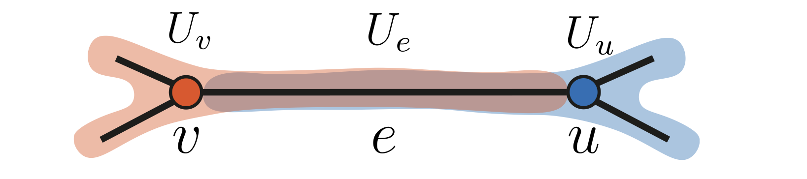
This defines a basis for a topology on a graph. It is easy to check why this is a basis.

Motivation

At this point, it is important to undeerstand the main issues in the current framework which is what we try to solve.

A main problem in machine learning, in the case of GNNs, is Node classificaiton. Given a feature, you would like to know which nodes have it, which do not. It has been concretely observed that GNNs face two issues trying to solve such a problem.

1) Oversmoothing: In general, the benefit of neural networks is their ability to understand complex behavior. The more layers you add, the more complicated problem they can handle. But that is not the case here, as yoou add more layers, the features of all nodes become progressively smoother and indistibguishable.

2) Heterophily Problem: Standard GNNs have a bias towards the hypothesis that all connected nodes belong to the sam class. This is called the homophily assumption. They thus break down when a graph exhibits heterophilicity.

Let us make connections between GCNs and Heat diffusion processes.

Let G be a graph with self loops, degree matrix $D$, adjacency matrix $A$, normalized laplacian $\Delta_0 = I - D^{-1/2}AD^{1/2}$, and node features $\mathbf{X} \in \mathbb{R}^{n \times d}$. The heat diffusion is in fact a simple process suffering from oversmoothing and heterophily: \(\dot{X}(t) = -\Delta_0X(t)\)

Discretizing this differential equation, we get

\[X(t + 1) = X(t) - \Delta_0X(t) = (1- \Delta_0)X_t\]

Here is the mathematical eqation for our GCNs:

\[GCN(X, A) = \sigma(D^{-1/2}AD^{-1/2}XW) = \sigma((I - \Delta_0)XW)\]

(This is essentially the definition of GCN networks, nothing fancy going on here. Just note that every neural network have different functions associated with them which determine the activations at each neuron. This is just that standard cookbook recipe variant for the neural networks called GCNs.)

Notice how strikingly similar they are! It thus makes sense why GCNs suffer from the two problems mentioned above.

To overcome the difficulties, we need to make the base diffusion model more powerful. Now comes sheaf into the picture.

Sheaves

Let us define a presheaf first. On a topological space, Ii is an assignment of some data to the open sets of that topological space $X$. Thus, each open set $U$ of $X$ is mapped to the data, which is an object of some category (for example, the category of sets).

In other words, $\mathfrak{f}: U \to \mathfrak{f}(U)$ is a presheaf.

A presheaf follows one property (as part of its defnition). To understand that property, let us define the restriction map as follows:

For each inclusion of open sets $V \to U$, a map $\mathfrak{f}_{VU}: \mathfrak{f}(U) -> \mathfrak{f}(V)$ is called a restriction map. This makes sense, linguistically speaking. $V$ is in $U$, so you just restrict the data to the smaller set and call the corresponding map a restriction map of the original map.

Here is the properties(really two), which a presheaf must follow, readers familiar with Category Theory may find it pretty motivated.

1) $\mathfrak{f}	_{WV} \cdot \mathfrak{f}	_{VU} = \mathfrak{f}	_{WU}$
2) $\mathfrak{f}	{UU} = \text{Id}{\mathfrak{f}(U)}$.

Thus, $\mathfrak{f}$ is really a functor, specifically called a contravariant functor (Again, just words, so feel free to ignore these).

Exmaple: Let $X = \mathbb{R}, \mathfrak{f}(U) = {f: U \to \mathbb{R}

f\text{ is continuous}}$, where the restriction map is the natural one. This is a presheaf.

This particular example follows two more nice properties, which makes it a sheaf. Here are the two additional properties a sheaf must satisfy:

1) (Gluing Property): If ${U_i}$ is an open cover of $X$ and we have corresponding elements of presheaf on each of the open sets (restricted to these sets) such that they agree on the intersection, then there is an element of the presheaf on $X$ such that its restriction on each of these open sets give those corresponding elemetns.

2) (Uniqueness/Locality) This global element is unique. Locally, speaking, if the open cover does not cover X, the global element need not be unique, but rather its restriction to each of the open sets needs to be unique.

An element of a sheaf is called a section of the sheaf.

Another example is a sheaf of vector fields over manifolds. The restriction maps are just restrictions of the vector field.

The key idea is that sheafs are about forming bigger data from smaller data.

Remark: An example of a presheaf that is not a sheaf is:

$\mathfrak{f}(U) = {f: U \to \mathbb{R}

f \text{ is a continuous bounded function}}$

We just need to glue infinitely many functions bounded over a subset of the real line to easily obtain an unounded function.

Another example is the sheaf of constant functions.

Inspired by the general methods of constructing sheaf structures on posets, we can build a sheaf structure on graphs with the topology generated by the basis of open stars of all vertices and edges.

Sheaves on Graphs

A $B$ - presheaf (base presheaf) is a presheaf where we care only about the basic open sets. More formally:

1) For each open set $U$, we have $\mathfrak{f}(U)$ in say, a category of sets. 2) For each $V \subset U$ of members of $B$, we have the corresponding restriction function following the usual properties.

Now, we can easily define $B$ - presheafs on graphs.

We can similarly define a $B$ - sheaf. It is a $B$ - presheaf satisfying the locality(uniqueness) and the gluing condition.

Now, we have a remarkable result:

Theorem: Any $B$ - presheaf on a graph with the topology generated by the open stars is a $B$ - sheaf.

The proof is easy to check. We now want a sheaf out of it.

It fascinatingly turns out that sheaves behave like linear operators, and this nice property largely motivates their definition. It is sufficient to specify how they behave on a basis to fully specify their behavior.

Theorem: A base sheaf on $X$ uniquely induces a sheaf on $X$ such that the base sheaf and the sheaf are canonically isomorphic.

Let $I(U) = {V

V \in B, V \subset U}$. Then the sections of the sheaf $\mathfrak{F}$ are constructed as:

\[\mathfrak{F}(U) = \{(s_V)_{V \in I(U)} \in \prod_{V\in I(U)}{\mathfrak{F}(V)}| \mathfrak{F}_{V, W}(s_V) = s_W, \forall W\subset U\}\]

Cellular Sheafs

As mentioned earlier, the functor can map to any category. Let us consider vector spaces instead of sets (of course, they are important because we love vector spaces in machine learning).

A cellular sheaf $(G, F)$ of vector spaces on an undirected graph $G = (V, E)$ consists of:

1) A vector space $F(v)$ for each $v \in V$. 2) A vector space $F(e)$ for each $e \in E$. 3) A linear map $F_{v \leq e}: F(v) \to F(e)$ for each incident $v \leq e$ node-edge pair.

The vector spaces are called stalks and the linear maps are called the restriction maps.

For a sheaf $(F, G)$ we define $0$-cochains $C^0(G; F) = \bigoplus_{v \in V}F(v)$ and $1$-cochains $C^1(G; F) = \bigoplus_{e \in E}F(e)$ (this is just a direct sum of vector spaces). This just gathers all the stalks into a vector space.

For some arbitrary choice of orientation for each edge $e = u \to v \in E$ define the coboundary map $\delta: C^0(G; F) \to C^1(G; F)$ by $\delta(x)e := F{v \leq e}x_v - F_{v\leq e}x_u$. This is the sheaf coboundary operator, acting like a covariant derivative. It is a linear transformation. This setup sorts of puts the geometry on the graph.

The boundary operators create a chain complex (take the analog with the DeRham Cohomology, which we see in calculus):

\(0 \to C_n(K,\mathbb{R}) \to ... C_k(K, \mathbb{R}) \to ... \to C_1(K, \mathbb{R}) \to C_0(K, \mathbb{R}) \to 0\) where the maps are the respective boundary operators. The boundary operator is also defined naturally.

The coboundary operator above creates the cochain complex. This defines a cohomology group $H^k(K, \mathbb{R}) := \ker \delta_k / \text{im } \delta_{k-1} \cong H_k(K, \mathbb{R})$.

The sheaf coboundary operator defines a cochain complex over the graph.

Sheaf Laplacian

The sheaf laplacian is the linear operator $\delta^T\delta$